Yiluan Song - Phenology sample data

Data prepared for Dr. Yang Chen’s class STATS605 in 2023 Fall, also good for others interested in exploring phenology data.

Data files and code for generating them can be found in this GitHub repo.

This blog gives some first steps reading and visualizing the data.

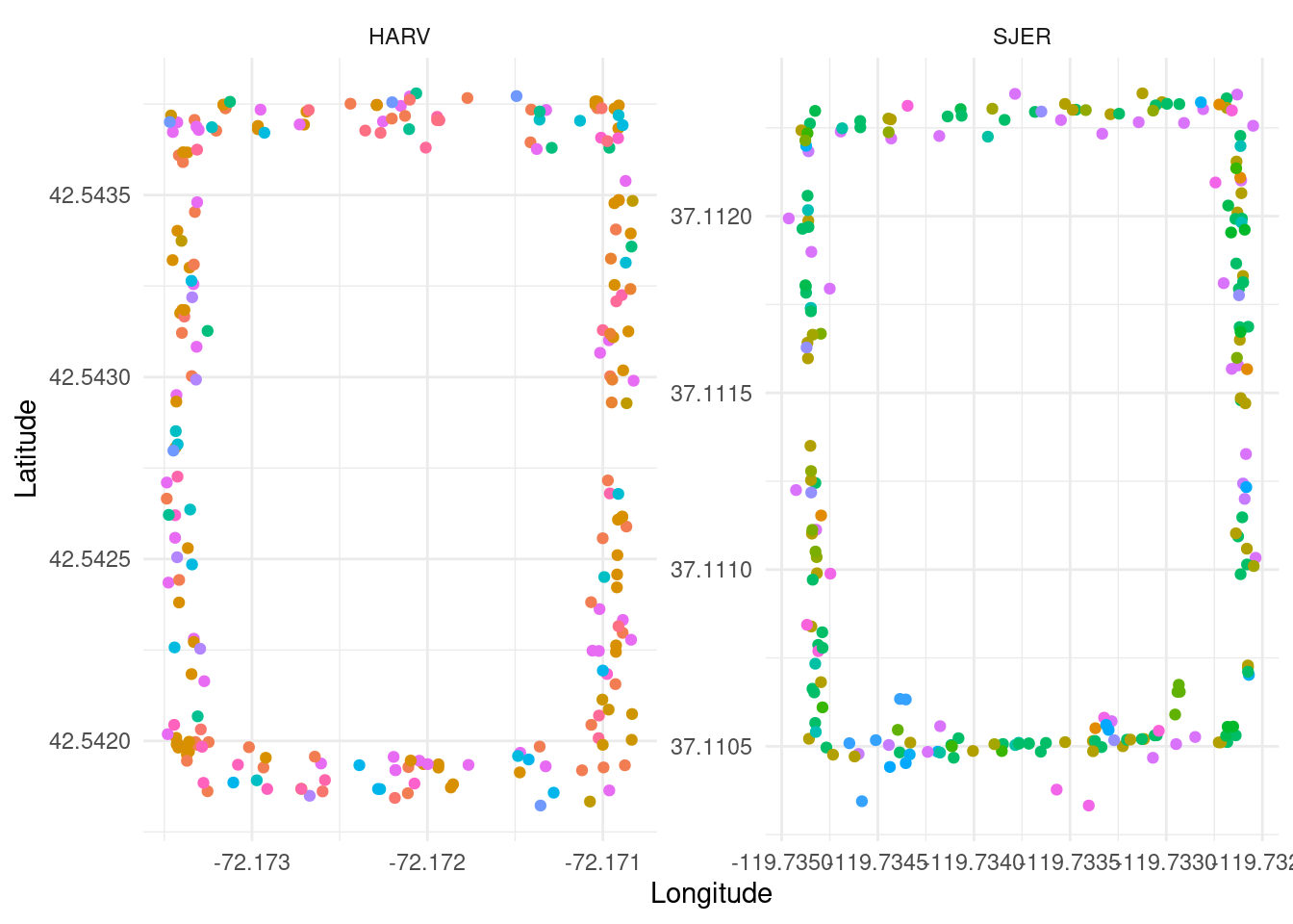
Meta data for trees

metadata <- read_csv("data/metadata.csv")

metadata %>%
  head() %>%
  flextable::regulartable() %>%
  flextable::autofit() %>%
  flextable::fit_to_width(8)

site	site_lat	site_lon	id	lat	lon	species	growth_form
HARV	42.54278	-72.17213	NEON.PLA.D01.HARV.06016	42.54368	-72.17330	Quercus rubra L.	Deciduous broadleaf
HARV	42.54278	-72.17213	NEON.PLA.D01.HARV.06046	42.54186	-72.17096	Quercus rubra L.	Deciduous broadleaf
HARV	42.54278	-72.17213	NEON.PLA.D01.HARV.06034	42.54310	-72.17097	Quercus rubra L.	Deciduous broadleaf
HARV	42.54278	-72.17213	NEON.PLA.D01.HARV.06041	42.54225	-72.17102	Quercus rubra L.	Deciduous broadleaf
HARV	42.54278	-72.17213	NEON.PLA.D01.HARV.06039	42.54233	-72.17089	Quercus rubra L.	Deciduous broadleaf
HARV	42.54278	-72.17213	NEON.PLA.D01.HARV.06029	42.54373	-72.17132	Quercus rubra L.	Deciduous broadleaf

metadata %>%
  ggplot() +
  geom_point(aes(x = lon, y = lat, col = species)) +
  facet_wrap(. ~ site, scales = "free") +
  theme_minimal() +
  theme(legend.position = "bottom") +
  guides(col = "none") +
  labs(
    x = "Longitude",
    y = "Latitude"
  )

Coordinates of tagged trees at two selected sites. Colors indicate species.

Discrete phenology data.

rnpn::npn_pheno_classes() %>%
  filter(id %in% 1:5) %>%
  select(id, name, description) %>%
  flextable::regulartable() %>%
  flextable::autofit() %>%
  flextable::fit_to_width(8)

id	name	description
1	Initial shoot or leaf growth	Initiation of seasonal vegetative growth
2	Young leaves or needles	Presence of foliage still in process of maturing
3	Leaves or needles	Presence of live foliage
4	Colored leaves or needles	Senescent coloring of foliage
5	Falling leaves or needles	Dropping of foliage

dat_discrete <- read_csv("data/discrete.csv")

dat_discrete %>%
  filter(status == "yes") %>%
  mutate(doy = date %>% lubridate::mdy() %>% lubridate::yday()) %>%
  arrange(phenophase_code) %>%
  mutate(phenophase = factor(phenophase, levels = unique(phenophase))) %>%
  ggplot() +
  geom_segment(aes(x = doy, xend = doy, y = 0, yend = 1), alpha = 0.01, col = "dark green") +
  facet_wrap(. ~ phenophase * site, ncol = 2) +
  theme_classic() +
  labs(
    x = "Day of year",
    y = ""
  ) +
  theme(axis.title.y = element_blank())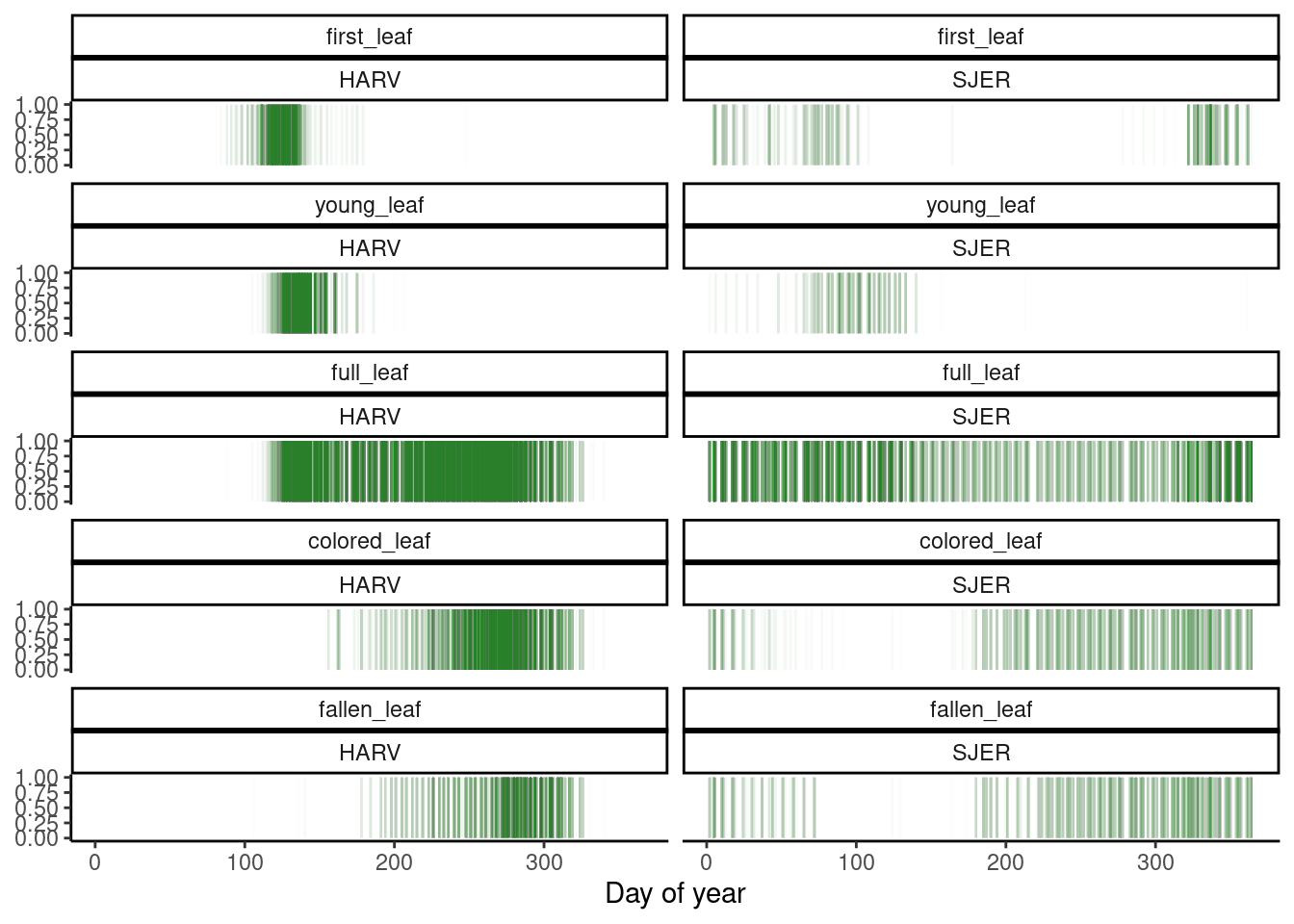

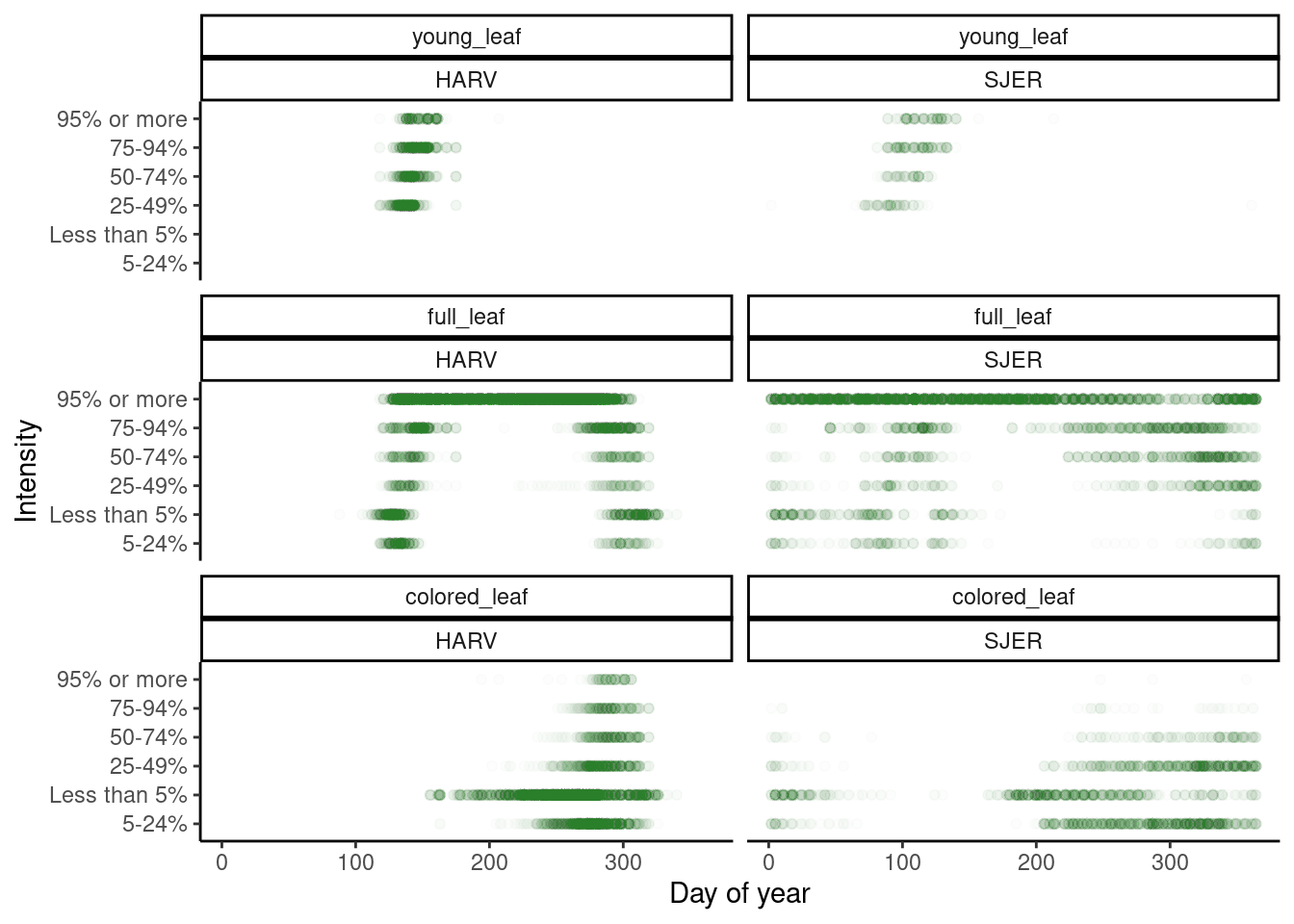
Time of Yes observation of phenophase status.

dat_discrete <- read_csv("data/discrete.csv")

dat_discrete %>%
  filter(!is.na(intensity)) %>%
  mutate(doy = date %>% lubridate::mdy() %>% lubridate::yday()) %>%
  arrange(phenophase_code) %>%
  mutate(phenophase = factor(phenophase, levels = unique(phenophase))) %>%
  arrange(intensity_code) %>%
  mutate(intensity = factor(intensity, levels = unique(intensity))) %>%
  ggplot() +
  geom_point(aes(x = doy, y = intensity), alpha = 0.01, col = "dark green") +
  facet_wrap(. ~ phenophase * site, ncol = 2) +
  theme_classic() +
  labs(
    x = "Day of year",
    y = "Intensity"
  )

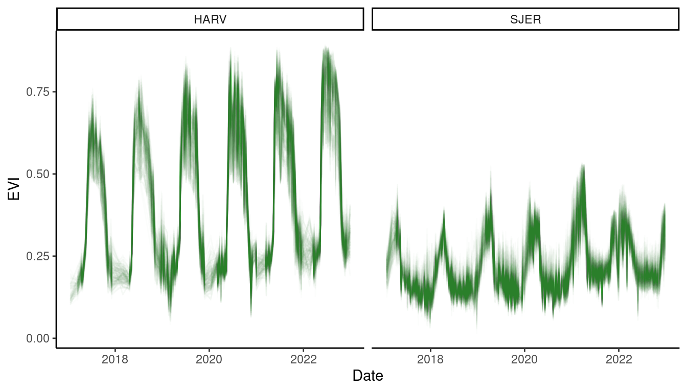
Continuous phenology data

dat_continuous_3m <- read_csv("data/continuous_3m.csv")

dat_continuous_3m %>%
  ggplot() +
  geom_line(aes(x = date, y = evi, group = id), alpha = 0.01, col = "dark green") +
  facet_wrap(. ~ site) +
  theme_classic() +
  labs(
    x = "Date",
    y = "EVI"
  )

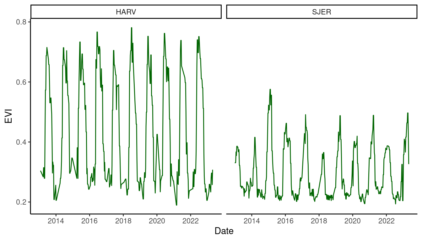
Enhanced vegetation index at 3 m resolution.

dat_continuous_500m <- read_csv("data/continuous_500m.csv")

dat_continuous_500m %>%
  ggplot() +
  geom_line(aes(x = date, y = evi), col = "dark green") +
  facet_wrap(. ~ site) +
  theme_classic() +
  labs(
    x = "Date",
    y = "EVI"
  )

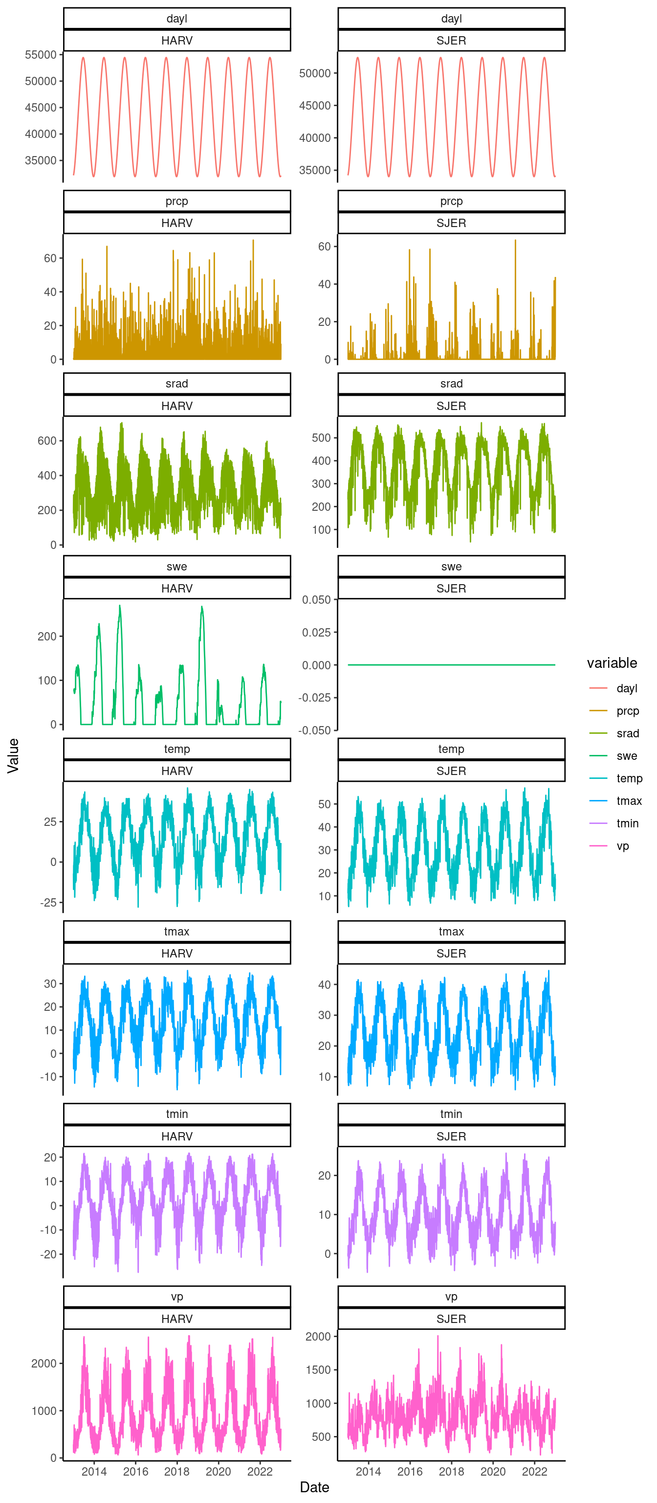
Enhanced vegetation index at 500 m resolution.

Weather data

dat_weather <- read_csv("data/weather.csv")

dat_weather %>%
  gather(key = "variable", value = "value", -site, -date) %>%
  ggplot() +
  geom_line(aes(x = date, y = value, col = variable)) +
  facet_wrap(. ~ variable * site, scales = "free_y", ncol = 2) +
  theme_classic() +
  labs(
    x = "Date",
    y = "Value"
  )